Regression analysis is a statistical tool used for decision-making and business forecasting.
According to YA-Lum-Chou, "Regression Analysis attempts to establish the nature of the relationship between variables that is to study the functional relationship between the variables and they're by providing a mechanism for prediction and forecasting".
Regression analysis studies the nature of the relationship between two variables so that we can estimate one variable against the variable.
Regression Example:
In a chemical process, suppose that the yield of the product is related to the process operating temperature. Regression analysis can be used to build a that expresses yield as a function of temperature. A regression model can be used to predict yield at a given temperature level. It could also be used for process optimization or process control purposes.
There is some basic concept of regression to understand before applying a regression line.
1. Nature of Relationship:
Regression means the act of return. It is a mathematical measure that shows the average relationship between two variables.
2. Forecasting:
Regression analysis enables to making of predictions. For example, by using regression equations x and y we can estimate the most probable value of x on the basis of the given value of y.
3. Cause and Effect:
Regression analysis clearly expresses the cause-and-effect relationship between two variables. It establishes
the functional relationship.Where one variable is treated as the dependent variable and another one is the independent variable.
4 Absolute and Relative Measurements:
The regression coefficient is an absolute measure. If we know the value of an independent variable. we can estimate the value of a dependent variable.
5. Effect of change in origin and scale:
Regression coefficients are independent of change in origin but not of change in scale.
6. Symmetry:
In regression analysis, it is required to be clearly identified which variable is the dependent variable and which one is independent. If b(xy) is not equal to b(yx), regression coefficients are not symmetric.
Regression is a statistical technique used for modeling and analyzing the relationship between one or more independent variables (predictors or features) and a dependent variable (the outcome or target). It aims to identify and quantify the nature of the relationship and make predictions or inferences based on this relationship. Regression analysis is widely used in various fields, including economics, finance, science, social sciences, and machine learning.
Key components and concepts of regression analysis include:
Dependent Variable (Y): This is the variable that you want to predict or explain. It is also referred to as the target variable or response variable. In a simple linear regression, there is only one dependent variable, while in multiple regression, there can be several.
Independent Variables (X): These are the variables that are used to predict or explain the dependent variable. They are also called predictors, features, or explanatory variables. In multiple regression, there are multiple independent variables.
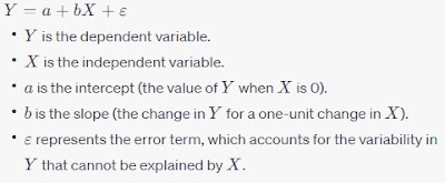
Regression Equation/Model: A regression equation or model is a mathematical representation of the relationship between the independent and dependent variables. In its simplest form, for a simple linear regression, it can be expressed as:
Regression Line
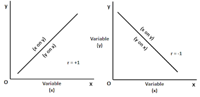
The regression line shows the average relationship between the two variables. There are two regression lines, namely regression lines of x on y and regression lines of y on x.On the basis of the regression line, we can predict the value of the dependent variable on the basis of the given value of the independent variable. It shows the average relationship between two variables is called the Line of Best Fit. Here we can estimate the value of x on the basis of a given value of y, otherwise, the value of y is on the basis of a given value of x.
If there is a perfect correlation between two variables x and y so that r = +1, r = -1 then there will be only one regression line. If the correlation is positive then the direction of the regression line will be upward from left to right. In the case of negative correlation, the line will slope down from left to right as shown in the figure
The important fact to be noted here is that either both lines will move from left to right or right to left. It is not possible that one will be left to right and another one is right to left.
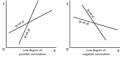
If two regression lines intersect each other at 90 degrees then it means that there is no correlation between the two variables so r= 0 is clear from the diagram given below.
Both the regression lines intersect each other at the point of average of x and y. If we draw a perpendicular from the point of intersection on the x-axis we will get the mean value of x and if we draw a perpendicular from the point of intersection from the y-axis we will get the mean value of y.
Regression Analysis Used
Regression analysis is used in economics, business research, and all scientific disciplines. In economics, it is used to estimate the relationship between variables like price and demand, income and saving, etc. If we know our income, we can estimate the probable savings. In business, we know that the quantity of scale is affected by the expenditure on advertisements like social media, etc. So a problem is based on a cause-and-effect relationship, the regression analysis is very useful.
Regression analysis is used to find out the standard error of estimate for regressions which is a measure of unexplained variation in the dependent variable. It is helpful to determine the reliability of the prediction made by using regression.
Regression analysis is used to estimate the value of the dependent variable against the given value of an independent variable. It describes the average relationship existing between two variables x and y. For example, a businessman can estimate the probable falls in demand if he decides to increase the price of a commodity.
Regression analysis is used to make predictions in policy making. On the basis of regression analysis, we can make predictions that provide a sound basis for policy formulation in the socio-economic field. We will see some examples to use software Python and R.
Regression analysis is used in machine-learning artificial intelligence, data science, cloud computing, security, etc. Interconnectivity and data explosion are realities that open a world of new opportunities for every business that can read and interpret data in real-time. Coming from a long and glorious past in the field of statistics, econometrics, linear regression, and its derived methods can provide you with simple reliable, and effective tools R and Python to learn from data and act on regression analysis. If carefully trained with the right data, linear regression analysis can compete well against the most complex artificial intelligence technologies, offering you unbeatable ease of implementation and scalability for increasingly large problems.
Regression analysis is used in data science to serve thousands of customers using your company's website every day. Using available information about customers in your data warehouse, in the advertising business, an application delivering targeted advertisement.
Regression analysis is used in e-commerce, a batch application filtering customers to make more relevant commercial offers an online app recommending products to buy on the basis of ephemeral data such as navigation records.
Regression analysis is also used in the credit and insurance business, an application selecting whether to proceed with online inquiries from users, basing its judgment on their credit rating and past relationship with the company.
Regression analysis is used in python for data science. It can work better than other platforms with in-memory data because of its minimal memory footprint and excellent memory management. The memory garbage collector will often save the day when you load, transform, dice, slice, save or discard data using the various reiterations of data wrangling.
Regression Line Equation
A regression Line Equation is the algebraic expression of a regression line. As there are two regression lines, there is two regression line equation:
1. Regression line equation of x on y. This equation is used to estimate the most probable value of 'x' against the given value of variable 'y'. Here:
'x' is the dependent variable and
'y' is an independent variable
2. Regression line equation of y on x.This regression equation is
used to estimate the most probable value of 'y' against the given
value of variable 'x'.Here:
'y' is a dependent variable and
'x' is an independent variable.
Types of Regression: There are different types of regression analysis, including:
Simple Linear Regression: One dependent variable and one independent variable.
Multiple Regression: One dependent variable and multiple independent variables.
Polynomial Regression: Fits a curved line to the data.
Logistic Regression: Used for binary classification problems.
Ridge, Lasso, and Elastic Net Regression: Used for regularization and variable selection in multiple regression.
Simple linear Regression
The relationship between a single regressor variable x and
a response variable y.The regressor variable x is assumed
to be a continuous mathematical variable, controllable by
the experimenter. Suppose that the true relationship between
y and x is a straight line and that the observation y at each
level of x is a random variable. Now the expected value
of y for each value of x is
E(y|x)=B0+B1x
Where the intercept B0 and the slope B1 are unknown constants.
Least Squares Lines
Experimental data produce points (x1,y1),......(xn,yn) that when graphed, seem to lie close to a line. We want to determine the parameters B0 and B1 that make the line as"close'' to the points as possible.
Suppose B0 and B1 are fixed and consider the line y=B0+B1x. Corresponding to each data point (xj,yj) there is a point(xj, B0+B1xj) on the line with the same x-coordinate. We call Yj the observed value of y and B0+B1xj the predicted y-value. The difference between an observed y-value and a predicted value is called a residual.
There are several ways to measure how "close" the line is to the data. The primarily because the mathematical calculations are simple to add the squares of the residuals. The least-squares line is the line y=B0+B1X that minimizes the sum of the squares of the residuals. This line is also called a line of regression of y on x because any error in the data is assumed to be only in the y-coordinates. The coefficients B0 and B1 of the line are called regression coefficients.
If the data points were on the line, the parameters B0 and B1 would satisfy the equations
Predicted y-value Observed y-value
B0+B1x1 = y1
B0+B1x2 = y2
. .
. .
B0+B1xn = yn
We can write this system as
XB=y, where X= [ 1 x1
1 x2
. .
. .
1 xn ],
B=[B0
B1],
y=[y1
y2
.
.
yn]
If the data points don't lie on a line, then there is no parameter B0, B1 for which the predicted y-values in XB equal the observed y-values in y, and XB=y has no solution. This is a least-squares problem, AX=b, with a different notation!
The square of the distance between the vectors XB and y is precisely the sum of the squares of the residuals. The B that minimizes this sum also minimizes the distance between XB and y. Computing the least-squares solution of XB=y is equivalent to finding the B that determines the least-squares line.
Question.
Find the equation y=B0+B1x of the least-squares line that best fits the data points(2,1),(5,2),(7,3),(8,3).
We assume that each observation,y can be described by the model
y=B0+B1x+e
Where e is a random error with mean zero and variance.The {e}
are also assumed to be uncorrelated random variables. The regression
model of a given equation involving only a single regressor variable
x is often called the simple linear regression model.
Analysis of residuals is frequently helpful in checking the assumption that the errors are NID(0, var) and in determining whether additional terms in the model would be useful. The experimenter can construct a frequency histogram of the residuals or plot them on a normal probability paper. If the error is NID(0, var), then approximately 95% of standardized residuals should fall in the interval(-2,2). Errors far outside this interval may indicate the presence of an outlier, that is an observation that is a type of the rest of the data. Various rules have been proposed for discarding outliers.
Multiple Regression
Suppose an experiment involves two independent variables-say, x1 and x2, and one dependent variable y. A simple equation to predict y from x1 and x2 has the form
y=B0+B1x1+B2x2..........(1)
A more general prediction equation might have the form
y=B0+B1x1+B2X2+B3x1^2+B4 x1 x2+B5x2^2.........(2)
This equation is used in geology, for instance, to model erosion surface, glacial cirques, soil PH, and other quantities. In such cases, the least-squares fit is called a trend surface. Both equations (1) and (2) lead to a linear model because they are linear in the unknown parameters. In general, a linear model will arise whenever y is to be predicted by an equation of the form
y=B0f0(x1x2)+B1f1(x1x2)+.............+Bkfk(x1x2)
with f0.....fk any sort of known functions and B0.....Bk unknown weight.
A multiple regression model that involves more than one regressor variable
is called a multiple regression model. As an example, suppose that
the effective life of a cutting tool depends on the cutting speed and
the tool angle. A multiple regression model that might describe this
relationship is:
y=B0+B1x1+B2x2+e
Where y represents the tool life,x1 represents the cutting speed and x2
represents the tool angle. This is a multiple linear regression model with
two regressors. A linear function of the unknown parametersB0, B1, and
B2.The model describes a plane in the two-dimensional x1,x2 space. The
parameter B0 defines the intercept of the plane. We sometimes called
and B2 partial regression coefficients, because B1 measures the expected
change in y per unit change in x1 when x2 is held constant and B2
measures the expected change in y per unit change in x2 when x1 is
held constant.
Multiple Regression Analysis
Multiple regression analysis is a logical extension of simple regression analysis. In this method, two or more independent variables are used to estimate the values of the dependent variable. Here average relationship among three or more variables is computed and it is used to forecast the value of the dependent variable on the basis of the given values of independent variables. For example, we can estimate the value of X1 where the values of X2 and X3 are given. There are three main objectives of multiple correlations and regression analysis:
a) To drive an equation that provides estimates of the dependent variable from values of two or more independent variables.
b) To measure the error of estimate involved in using this regression equation as the basis of estimation.
c) To measure the proportion of variance in the dependent variable which is explained by dependent variables.
Regression Analysis Python
import pandas as pd
from sklearn.datasets import load_iris
data = load_iris()
iris = pd.DataFrame
(data.data, columns=data.feature_names)
iris.head()
sepal length (cm) | sepal width (cm) | petal length (cm) | petal width (cm) | |
|---|---|---|---|---|
0 | 5.1 | 3.5 | 1.4 | 0.2 |
1 | 4.9 | 3.0 | 1.4 | 0.2 |
2 | 4.7 | 3.2 | 1.3 | 0.2 |
3 | 4.6 | 3.1 | 1.5 | 0.2 |
4 | 5.0 | 3.6 | 1.4 | 0.2 |
iris['sepal length (cm)']
0 5.1
1 4.9
2 4.7
3 4.6
4 5.0
...
145 6.7
146 6.3
147 6.5
148 6.2
149 5.9
Name: sepal length (cm), Length: 150, dtype: float64
iris['sepal width (cm)']>1
0 True
1 True
2 True
3 True
4 True
...
145 True
146 True
147 True
148 True
149 True
Name: sepal width (cm), Length: 150,
dtype: bool
iris['petal width (cm)']>3
0 False
1 False
2 False
3 False
4 False
...
145 False
146 False
147 False
148 False
149 False
Name: petal width (cm), Length: 150,
dtype: bool
from matplotlib import pyplot as plt
import seaborn as sns
sns.scatterplot(x='sepal length (cm)',
y='petal length (cm)',data=iris)
y=iris[['sepal length (cm)']]
x=iris[['sepal width (cm)']]
from sklearn.model_selection
import train_test_split
x_train,x_test,y_train,y_test=
train_test_split
(x,y,test_size=0.3)
x_test.head()
| sepal width (cm) | |
|---|---|
| 17 | 3.5 |
| 112 | 3.0 |
| 26 | 3.4 |
| 31 | 3.4 |
| 80 | 2.4 |
x_train.head()
| sepal width (cm) | |
|---|---|
| 134 | 2.6 |
| 51 | 3.2 |
| 120 | 3.2 |
| 19 | 3.8 |
| 70 | 3.2 |
from sklearn.linear_model import
LinearRegression
lr=LinearRegression()
lr.fit(x_train,y_train)
LinearRegression(copy_X=True,
fit_intercept=True, n_jobs=None,
normalize=False)
y_pred=lr.predict(x_test)
y_test.head()
| sepal length (cm) | |
|---|---|
| 17 | 5.1 |
| 112 | 6.8 |
| 26 | 5.0 |
| 31 | 5.4 |
| 80 | 5.5 |
y_pred[0:5]
array([[5.68319154],
[5.84032627],
[5.71461848],
[5.71461848],
[6.02888794]])
from sklearn.metrics
import mean_squared_error
mean_squared_error(y_test,y_pred)
0.9060450498564653
y= iris[['sepal length (cm)']]
x=iris[['sepal width (cm)','petal length
(cm)','petal width (cm)']]
x_train,x_test,y_train,y_test=
train_test_split
(x,y,test_size=0.3)
x_train.head()
| sepal width (cm) | petal length (cm) | petal width (cm) | |
|---|---|---|---|
| 99 | 2.8 | 4.1 | 1.3 |
| 82 | 2.7 | 3.9 | 1.2 |
| 69 | 2.5 | 3.9 | 1.1 |
| 148 | 3.4 | 5.4 | 2.3 |
| 135 | 3.0 | 6.1 | 2.3 |
lr2=LinearRegression()
lr2.fit(x_train,y_train)
LinearRegression(copy_X=True,
fit_intercept=True, n_jobs=None,
normalize=False)
y_pred=lr2.predict(x_test)
mean_squared_error(y_test,y_pred)
0.0813243348427029
# modle 2 is better than model 1
because a less mean square error is good


0 Comments